
机器学习--线性单元回归--单变量梯度下降的实现 【线性回归】 如果要用一句话来解释线性回归是什么的话,那么我的理解是这样子的: **线性回归,是从大量的数据中找出最优的线性(y=ax+b)拟合函数,通过数据确定函数中的未知参数,进而进行后续操作(预测) **回归的概念是从统计学的角度得出的,用抽样数据去预估整体(回归中,是通过数据去确定参数),然后再从确定的函数去预测样本。 【损失函数】
用线性函数去拟合数据,那么问题来了,到底什么样子的函数最能表现样本?对于这个问题,自然而然便引出了损失函数的概念,损失函数是一个用来评价样本数据与目标函数(此处为线性函数)拟合程度的一个指标。我们假设,线性函数模型为:

基于此函数模型,我们定义损失函数为:
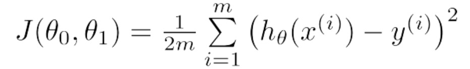
从上式中我们不难看出,损失函数是一个累加和(统计量)用来记录预测值与真实值之间的1/2方差,从方差的概念我们知道,方差越小说明拟合的越好。那么此问题进而演变称为求解损失函数最小值的问题,因为我们要通过样本来确定线性函数的中的参数θ_0和θ_1. 【梯度下降】
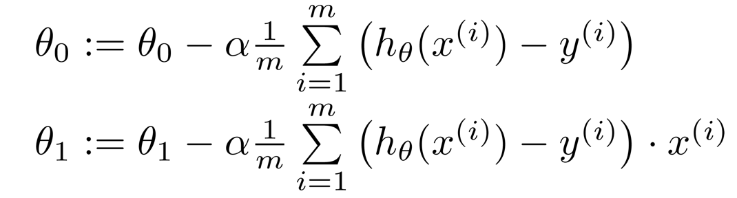
梯度下降算法是求解最小值的一种方法,但并不是唯一的方法。梯度下降法的核心思想就是对损失函数求偏导,从随机值(任一初始值)开始,沿着梯度下降的方向对θ_0和θ_1的迭代,最终确定θ_0和θ_1的值,注意,这里要同时迭代θ_0和θ_1(这一点在编程过程中很重要),具体迭代过程如下:
那么下面我们使用python代码来实现线性回归的梯度下降。
#此处数据集,采用吴恩达第一次作业的数据集:ex1data1.txt # -*- coding: utf-8 -*- import numpy as np import matplotlib.pyplot as plt # 读取数据 def readData(path): data = np.loadtxt(path, dtype=float, delimiter=',') return data # 损失函数,返回损失函数计算结果 def costFunction(theta_0, theta_1, x, y, m): predictValue = theta_0 + theta_1 * x return sum((predictValue - y) ** 2) / (2 * m) # 梯度下降算法 # data:数据 # theta_0、theta_1:参数θ_0、θ_1 # iterations:迭代次数 # alpha:步长(学习率) def gradientDescent(data, theta_0, theta_1, iterations, alpha): eachIterationValue = np.zeros((iterations, 1)) x = data[:, 0] y = data[:, 1] m = data.shape[0] for i in range(0, iterations): hypothesis = theta_0 + theta_1 * x temp_0 = theta_0 - alpha * ((1 / m) * sum(hypothesis - y)) temp_1 = theta_1 - alpha * (1 / m) * sum((hypothesis - y) * x) theta_0 = temp_0 theta_1 = temp_1 costFunction_temp = costFunction(theta_0, theta_1, x, y, m) eachIterationValue[i, 0] = costFunction_temp return theta_0, theta_1, eachIterationValue if __name__ == '__main__': data = readData('ex1data1.txt') iterations = 1500 plt.scatter(data[:, 0], data[:, 1], color='g', s=20) # plt.show() theta_0, theta_1, eachIterationValue = gradientDescent(data, 0, 0, iterations, 0.01) hypothesis = theta_0 + theta_1 * data[:, 0] plt.plot(data[:, 0], hypothesis) plt.title("Fittingcurve") plt.show() plt.plot(np.arange(iterations),eachIterationValue) plt.title('CostFunction') plt.show() # 在这里我们使用向量的知识来写代码 # -*- coding: utf-8 -*- import numpy as np import matplotlib.pyplot as plt """ 1.获取数据,并且将数据变为我们可以方便使用的数据格式 """ def LoadFile(filename): data = np.loadtxt(filename, delimiter=',', unpack=True, usecols=(0, 1)) X = np.transpose(np.array(data[:-1])) y = np.transpose(np.array(data[-1:])) X = np.insert(X, 0, 1, axis=1) m = y.size return X, y, m """ 定义线性关系:Linear hypothesis function """ def h(theta, X): return np.dot(X, theta) """ 定义CostFunction """ def CostFunction(theta, X, y, m): return float((1. / (2 * m)) * np.dot((h(theta, X) - y).T, (h(theta, X) - y))) iterations = 1500 alpha = 0.01 def descendGradient(X, y, m, theta_start=np.array(2)): theta = theta_start CostVector = [] theta_history = [] for i in range(0, iterations): tmptheta = theta CostVector.append(CostFunction(theta, X, y, m)) theta_history.append(list(theta[:, 0])) # 同步更新每一个theta的值 for j in range(len(tmptheta)): tmptheta[j] = theta[j] - (alpha / m) * np.sum((h(theta, X) - y) * np.array(X[:, j]).reshape(m, 1)) theta = tmptheta return theta, theta_history, CostVector if __name__ == '__main__': X, y, m = LoadFile('ex1data1.txt') plt.figure(figsize=(10, 6)) plt.scatter(X[:, 1], y[:, 0], color='red') theta = np.zeros((X.shape[1], 1)) theta, theta_history, CostVector = descendGradient(X, y, m, theta) predictValue = h(theta, X) plt.plot(X[:, 1], predictValue) plt.xlabel('the value of x') plt.ylabel('the value of y') plt.title('the liner gradient descend') plt.show() plt.plot(range(len(CostVector)), CostVector, 'bo') plt.grid(True) plt.title("Convergence of Cost Function") plt.xlabel("Iteration number") plt.ylabel("Cost function") plt.xlim([-0.05 * iterations, 1.05 * iterations]) plt.ylim([4, 7]) plt.title('CostFunction') plt.show() # 我们使用我们写好的线性模型去预测未知数据的情况,这样我们就可以得出一个属于我们自己的结果。 # 把我们线性模型预测的结果和实际的结果作一个对比,我们就可以看出实际结果是否真假性。 X, y, m = LoadFile('ex1data3.txt') predictValue = h(theta, X) print(predictValue) # 这里我们可以得到我们的预测值,我们用建立好的模型去预测未知的模型情况。 ‘’‘ [[1.16037866] [3.98169165]] ’‘’项目运行的结果为: